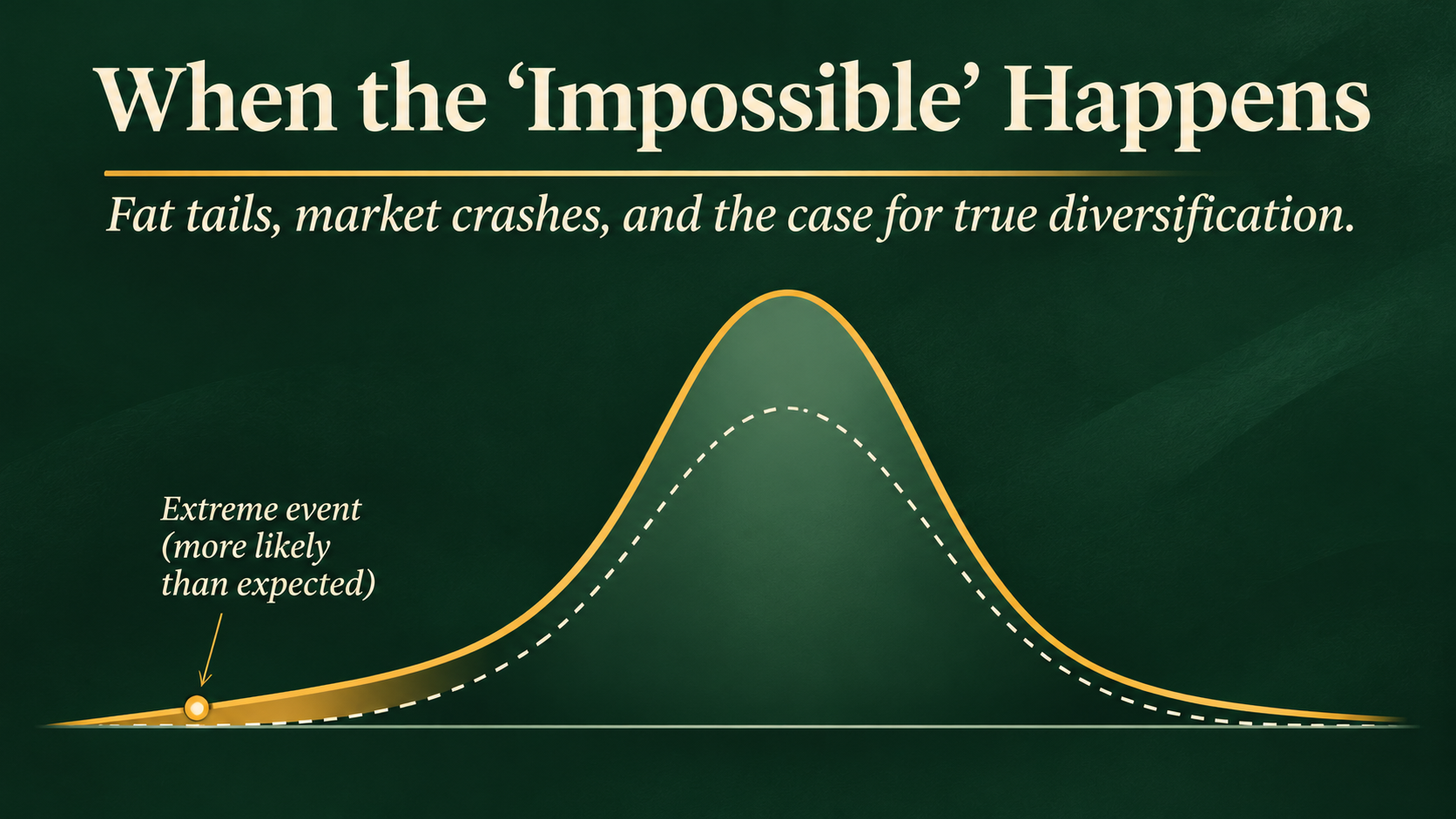
Financial markets regularly experience events that conventional statistical models suggest should almost never happen. From Brazil’s 2026 market collapse to Wall Street’s Black Monday, these supposedly impossible events reveal a fundamental weakness in how investors understand risk – and why genuine diversification matters.
A Market Crash That Shouldn’t Have Happened for Billions of Years
On 26 October 2026, Brazilian equities experienced a historic selloff.
Following the unexpected re-election of President Luiz Inácio Lula da Silva, the dollar-denminated iShares MSCI Brazil ETF (ticker: EWZ) plunged 19.8% in a single trading session. The ETF briefly traded more than 26% below its previous closing price.
For investors who had positioned themselves for a different election outcome, the losses were devastating.
But there was something even more remarkable about the decline.
Using a historical average daily return of approximately 0.04% and standard deviation of 2.36%, the decline represented an event of roughly 8.4 standard deviations, or sigma, below the mean.
Under the assumption that daily market returns follow a normal, or Gaussian, distribution, the probability of such an event is extraordinarily small.
An 8.4-sigma negative event has a theoretical one-day probability of roughly one in several quadrillions – or once every 150 billion years.
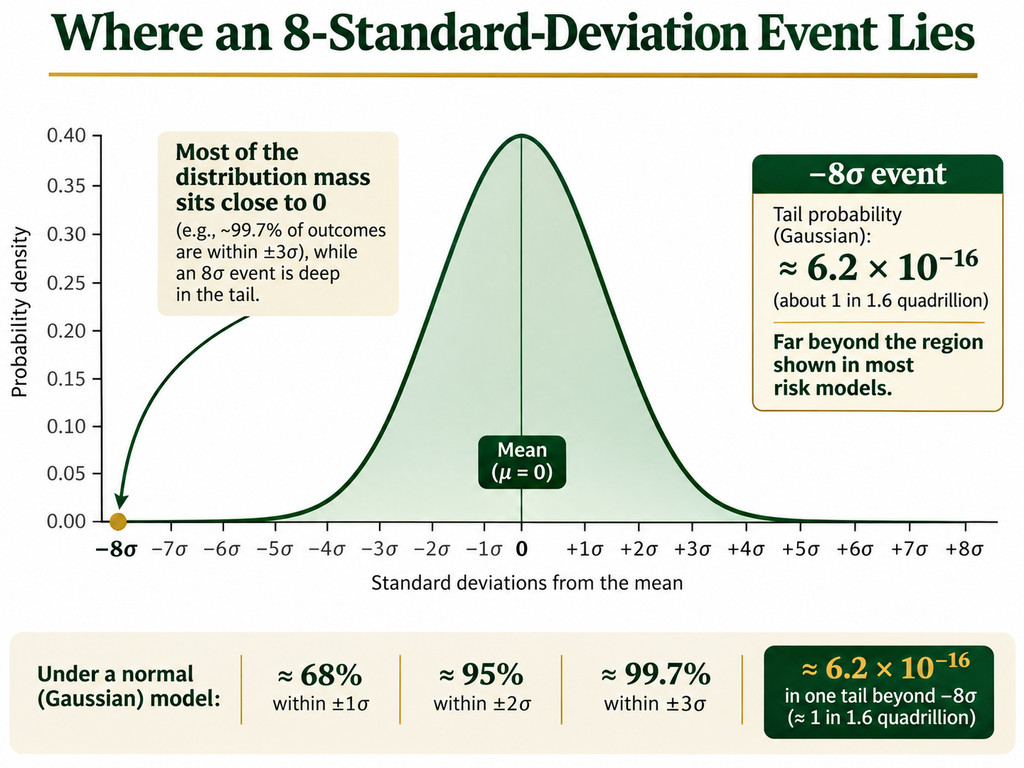
Depending on the assumptions used, calculations of extreme market events can produce expected waiting times ranging from billions of years to vastly longer than the age of the universe.
Yet something resembling this supposedly impossible event had already happened in Brazil.
Twice.
| Date | EWZ daily decline | Context |
|---|---|---|
| 15 October 2008 | −19.6% | Global financial crisis |
| 16 March 2020 | −23.1% | COVID-19 market crash |
| 26 October 2026 | −19.8% | Brazilian presidential election |
Three single-day declines of approximately 20% or more in just 18 years.
And all three occurred within the ETF’s relatively short history. The figures were documented in ETF.com’s coverage of Brazil’s October 2026 crash.
These types of comments of a one-in-a-billion-crashes are often regurgitated in both social media and the financial (and even regular) press in connection to steep declines. While such headlines generate clicks and interest, there is something profoundly inaccurate around such simplistic prose.
Of course, the precise Gaussian probability depends on the volatility estimation period, return definition, and other assumptions. The calculation above is illustrative rather than a calibrated forecast, and the three observations do not all have identical statistical magnitudes.
Nevertheless, the contradiction is striking.
When an event that supposedly shouldn’t happen for billions of years occurs repeatedly within a generation, perhaps the problem isn’t the market. Perhaps it’s the model.
The Beautiful Simplicity – and Dangerous Limitations – of the Bell Curve
Much of modern financial risk management is built around statistical concepts that work remarkably well in many areas of science.
One of the most familiar is the normal distribution, commonly called the bell curve.
In a normal distribution, observations cluster around an average. Small deviations are common, while increasingly large deviations become exponentially less likely.
For a normally distributed variable:
- Approximately 68% of observations fall within one standard deviation of the mean.
- Approximately 95% fall within two standard deviations.
- Approximately 99.7% fall within three standard deviations.
- Events beyond five or six standard deviations become exceptionally rare.
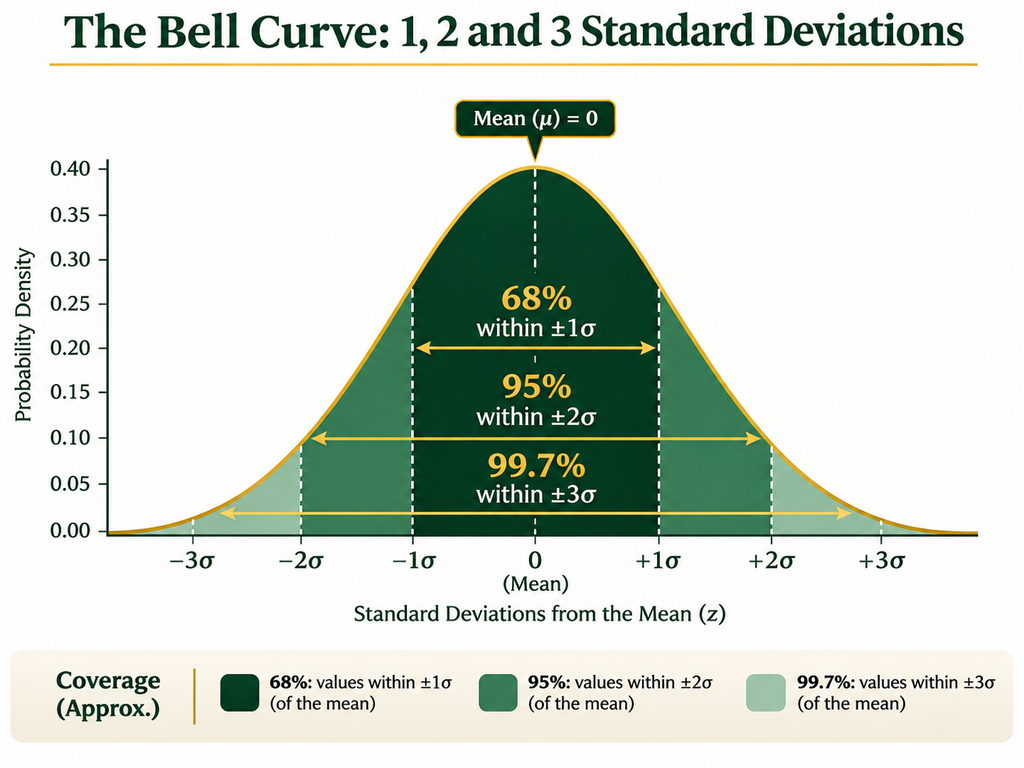
Applied to investing, this framework allows analysts to estimate the probability of different returns based on historical averages and volatility.
It is mathematically elegant, computationally convenient, and often useful for understanding ordinary market fluctuations.
The problem arises when investors assume that this approximation accurately describes extreme market behaviour.
Financial returns frequently exhibit what statisticians call fat tails.
In a fat-tailed distribution, unusually large positive and negative outcomes occur more frequently than the normal distribution predicts.
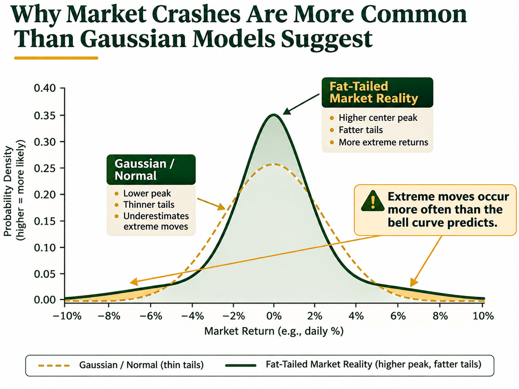
Markets also exhibit volatility clustering: periods of relative calm tend to be followed by more calm, while turbulent periods often produce additional turbulence.
In other words, market volatility is neither constant nor independent of previous observations.
A large market decline can itself change investor behaviour, liquidity conditions, and the probability of further declines.
These characteristics violate some of the simplifying assumptions behind conventional Gaussian risk models.
The normal distribution isn’t mathematically wrong.
It is simply not a sufficiently accurate description of how financial markets behave, particularly at the extremes.
This distinction matters enormously.
A model that performs reasonably well 99% of the time may still be dangerously misleading if its errors are concentrated in the remaining 1% – precisely when investors face their largest potential losses.
Wall Street Has Seen the “Impossible” Before
Brazil in October 2026 is far from an isolated example.
Some of the most famous episodes in financial history demonstrate the limitations of assuming that market returns behave normally.
Black Monday, 1987: A Crash Beyond Imagination
On 19 October 1987, the Dow Jones Industrial Average plunged 22.6% in a single trading session.
It remains the largest one-day percentage decline in the index’s history.
Depending on the historical volatility estimate used, the crash has been described as an event exceeding 20 standard deviations.
Under a normal distribution, the theoretical probability of such an observation is effectively zero on any meaningful human timescale.
Yet it happened.
The explanation was not a single unprecedented economic catastrophe.
Instead, a combination of market uncertainty, declining liquidity, interconnected trading strategies, and portfolio insurance mechanisms amplified selling pressure.
As markets fell, strategies designed to reduce exposure generated additional selling.
That selling pushed prices lower, triggering further selling.
The result was a self-reinforcing feedback loop.
The Federal Reserve’s historical account of Black Monday describes how interconnected markets and trading behaviour contributed to the collapse.
The lesson extends well beyond 1987. Markets are not collections of independent random observations.
They are complex systems in which participants respond to one another, often in ways that amplify extreme outcomes.
The 2007 Quantitative Meltdown: When Sophisticated Models Failed Together
Twenty years later, another extraordinary episode exposed similar weaknesses.
During August 2007, several prominent quantitative investment funds experienced severe losses as previously successful trading strategies abruptly broke down.
Goldman Sachs’ chief financial officer, David Viniar, famously described the market movements as 25-standard-deviation events occurring on several consecutive days.
The statement attracted considerable attention.
A genuine 25-sigma event under a Gaussian distribution is so improbable that observing several in succession would be practically inconceivable.
But the market movements were real.
The underlying problem was that numerous sophisticated investment strategies had become exposed to similar risks.
Funds were holding overlapping positions, employing leverage, and relying on historical relationships that appeared relatively stable.
When some investors were forced to reduce their exposures, selling pressure affected other funds holding similar positions.
Historical correlations became unreliable as previously distinct strategies suffered simultaneous losses.
The episode demonstrated an uncomfortable truth:
Sophisticated statistical models do not necessarily produce sophisticated risk management.
If many investors use similar models, their collective behaviour can create precisely the risks those models fail to anticipate.
The events were documented in contemporary financial reporting and subsequently examined in research on quantitative investment strategies.
Different Crises, Similar Lessons
The 1987 crash, the 2007 quantitative meltdown, the 2008 financial crisis, the 2020 pandemic shock, and Brazil’s 2026 election selloff had very different catalysts.
Yet they share important characteristics.
Investors underestimated the potential magnitude of losses, historical relationships proved unreliable, and market reactions were amplified by changing expectations, liquidity, positioning, or forced selling.
These episodes should not be interpreted as identical statistical events. They involved different assets, volatility regimes, and market structures.
What connects them is the broader failure of models that assume the future will resemble a relatively stable extrapolation of the past.
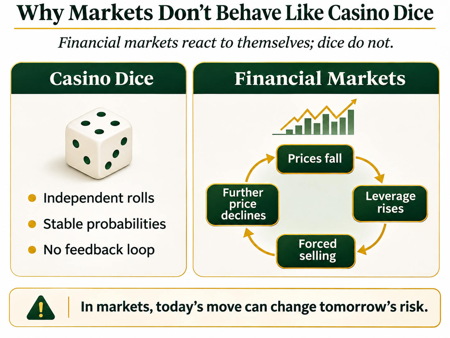
Why Markets Don’t Behave Like Casino Dice
One reason Gaussian assumptions can be misleading is that financial markets are fundamentally different from many of the physical processes where normal distributions work well.
Consider rolling a fair die.
The probability of rolling a six does not change because the previous ten rolls happened to produce sixes.
Financial markets are different.
Investors observe prices, form expectations, respond to economic developments, and adjust their positions.
Those decisions influence prices, which in turn influence other investors’ decisions.
The system continuously reacts to itself.
Consider a simplified example.
An investment fund uses leverage to increase its exposure to equities.
During normal market conditions, the strategy generates attractive returns.
But when equities begin falling, the fund’s leverage increases relative to its remaining capital.
To maintain its risk limits, it must sell assets.
If numerous funds face similar constraints, they may all attempt to sell simultaneously.
The resulting selling pressure causes further price declines, forcing additional deleveraging.
An initially manageable market movement can therefore become a much larger event.
This is one reason financial crises frequently involve abrupt changes in correlations and liquidity.
Assets that previously appeared relatively independent can suddenly move together.
Not necessarily because their underlying economic fundamentals have changed equally, but because investors are responding to common financial constraints.
Risk is not merely a statistical property of individual assets. It is also a consequence of how investors, institutions, and markets interact.
The Hidden Risk of Investing in Just One Market
For individual investors, the implications are particularly important.
Many investors believe they are adequately diversified because they own an index fund containing hundreds of companies.
An investor holding a broad Brazilian equity fund, for example, owns businesses across several sectors.
That reduces exposure to the fortunes of any single company.
But it does not eliminate exposure to Brazil’s broader economic and political environment.
Changes in fiscal policy, interest rates, currency expectations, or investor confidence can affect many Brazilian companies simultaneously.
The October 2026 collapse illustrated this concentration of risk.
Investors holding the EWZ ETF suffered a loss of almost 20% in one day, despite owning a diversified portfolio of Brazilian equities.
The fund diversified company-specific risk.
It did not diversify away country risk.
The same principle applies to developed markets.
An investor holding only an S&P 500 index fund has substantial diversification across American companies.
However, the portfolio remains overwhelmingly exposed to equity-market risk.
If investors collectively demand a higher risk premium for owning stocks, or if corporate earnings expectations deteriorate, a large proportion of those companies may decline together.
Geographic diversification can help, but it is not always sufficient.
During global financial crises, equity markets across different countries often become more strongly correlated.
An investor holding American, European, and Japanese equity funds may therefore discover that the apparent diversification provides less protection than expected.
This does not make equity index funds unsuitable investments.
For many investors, they are efficient, inexpensive vehicles for long-term wealth accumulation.
However, diversification across companies is not the same as diversification across economic risks.
That distinction is fundamental to constructing a resilient portfolio.
Why Traditional Diversification Can Disappoint
One of the most familiar investment portfolios is the traditional 60/40 allocation.
It combines 60% equities with 40% bonds.
Historically, this approach has often provided a reasonable balance between growth and stability.
Equities offer exposure to corporate earnings and economic expansion, while high-quality government bonds have frequently performed well during growth-driven recessions.
However, this relationship is not guaranteed.
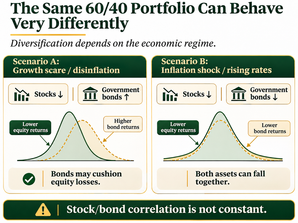
Consider two different economic scenarios.
Scenario A: Economic growth collapses.
Corporate earnings expectations deteriorate, causing equities to decline.
Central banks may respond by lowering interest rates.
Falling interest rates generally increase the market value of existing fixed-rate bonds, particularly those with longer maturities.
In this environment, equities and government bonds may offset one another.
Scenario B: Inflation unexpectedly accelerates.
Central banks may be forced to raise interest rates.
Higher discount rates can pressure equity valuations, while rising bond yields cause existing bonds to lose value.
Both asset classes can therefore decline simultaneously.
A portfolio that appeared diversified under the first scenario may perform poorly under the second.
This was an important feature of the market environment in 2022, when inflation and rising interest rates placed pressure on both stocks and bonds.
The underlying issue is not that bonds have suddenly stopped being useful.
Rather, the relationship between stocks and bonds depends on the economic environment.
A portfolio manager who assumes that historical correlations are permanent may be overlooking one of the most important sources of portfolio risk.
Correlation Is Not a Constant
Correlation measures the extent to which two assets tend to move together.
A correlation of +1 indicates perfectly aligned movements, while −1 indicates perfectly opposite movements.
A correlation near zero indicates little linear relationship.
These statistics are useful when constructing portfolios.
But correlations are not fixed characteristics of financial assets.
They can change substantially as economic conditions evolve.
Stocks and bonds may exhibit negative correlations during periods dominated by growth uncertainty.
They may become positively correlated when inflation and monetary tightening dominate.
Similarly, assets that appear unrelated during normal conditions may suddenly become correlated during liquidity crises.
A portfolio manager should therefore distinguish between two questions:
- How have these assets behaved together historically?
- Why should we expect them to behave differently under particular future economic conditions?
The second question is arguably more important.
Historical correlations describe what happened.
Economic reasoning helps us understand what might happen when the environment changes.
This does not mean abandoning quantitative analysis.
It means using quantitative analysis alongside a coherent understanding of the economic forces driving asset returns.
Understanding Cross-Asset Dependencies
Consider a portfolio containing equities, government bonds, gold, and commodities.
Each asset has different sensitivities to economic developments.
Equities generally benefit from stronger corporate earnings and economic growth.
Nominal government bonds are sensitive to interest rates, inflation expectations, and monetary policy.
Gold responds to several forces, including real interest rates, currency developments, and demand for defensive assets.
Broad commodity exposure is influenced by supply and demand, inflationary pressures, and economic activity.
These relationships are not universal or stable.
For example, gold can decline during a liquidity crisis if investors sell liquid assets to raise cash.
Government bonds can suffer substantial losses when inflation expectations rise.
Commodities can fall sharply during demand-driven recessions.
Nevertheless, the underlying economic exposures differ sufficiently to create opportunities for meaningful diversification.
A thoughtful portfolio manager should examine these relationships rather than relying exclusively on historical volatility and correlation estimates.
The All-Seasons Approach: Diversifying Across Economic Environments
This brings us to the central philosophy behind an All-Seasons Portfolio.
Rather than attempting to predict the next market crash, the objective is to construct a portfolio that is reasonably resilient across a wide range of economic outcomes.
The starting point is simple:
We cannot consistently predict the future economic environment, but we can prepare for several different possibilities.
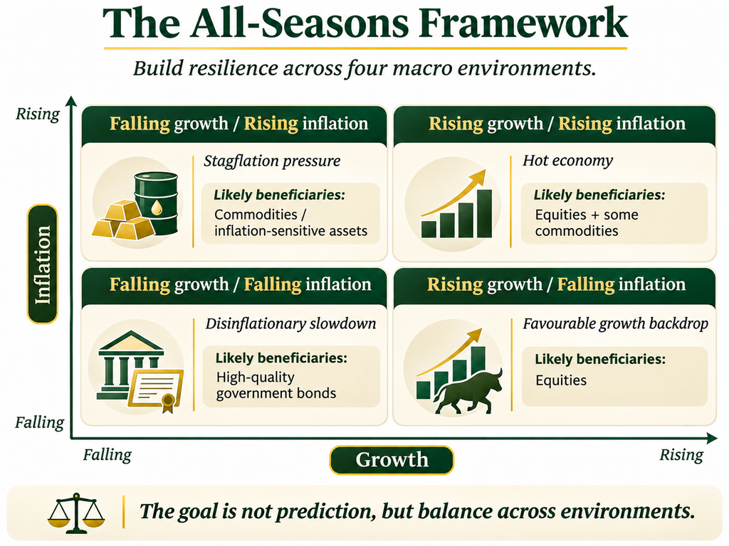
One useful framework considers two fundamental economic variables:
- Economic growth, which can exceed or fall short of expectations.
- Inflation, which can exceed or fall short of expectations.
Combining these variables produces four broad economic environments.
| Economic environment | Typical characteristics | Assets that may benefit |
|---|---|---|
| Rising growth, falling inflation | Strong economic activity and favourable financial conditions | Equities |
| Rising growth, rising inflation | Economic expansion accompanied by inflationary pressures | Equities and certain commodities |
| Falling growth, falling inflation | Disinflationary slowdown or recession | High-quality government bonds |
| Falling growth, rising inflation | Stagflationary conditions | Certain commodities, gold and inflation-sensitive assets |
These are simplified relationships, not guaranteed outcomes.
Nevertheless, they provide an economically grounded framework for portfolio construction.
Instead of concentrating capital in whichever asset class has performed best recently, an All-Seasons strategy seeks exposure to assets that respond differently to changes in growth and inflation.
The objective is not to eliminate losses.
No realistic portfolio can provide positive returns under every conceivable scenario.
Rather, the goal is to reduce dependence on any single economic outcome.
Why Risk Matters More Than Capital Allocation
A further consideration is that allocating equal amounts of capital does not necessarily produce equal amounts of risk.
Suppose a portfolio invests 50% in equities and 50% in government bonds.
If equities are substantially more volatile than bonds, they may account for the overwhelming majority of the portfolio’s overall risk, as we have discussed in another article about why the 60/40 Portfolio is not balanced.
The portfolio may therefore be far less balanced than its capital weights suggest.
Risk parity approaches address this problem by considering the contribution of different assets to total portfolio risk.
The aim is to avoid allowing one asset class to dominate the portfolio simply because it has higher volatility.
However, risk parity is not a magic formula.
Risk contributions depend on estimated volatilities and correlations, which can change.
Some implementations also use leverage, introducing financing costs, liquidity considerations, and additional risks.
A robust approach therefore combines risk balancing with an understanding of the underlying economic exposures.
The objective should not be mathematical perfection, but sensible diversification across genuinely different sources of risk.
What Smart Portfolio Management Looks Like
If extreme market events are more common than conventional models suggest, how should investors respond?
The answer is not to abandon statistical analysis.
Nor is it to assume that another market crash is always imminent.
Instead, investors should adopt a more realistic framework for understanding uncertainty.
1. Treat Historical Volatility as an Estimate, Not a Boundary
An asset with historically low volatility is not necessarily safe.
Volatility measures observed fluctuations over a particular period.
It does not establish a maximum possible loss.
A prolonged period of stability may even encourage investors to increase leverage or concentrate their positions, making the system more vulnerable to unexpected shocks.
Risk assessments should therefore consider outcomes beyond those observed in recent history.
That’s why most All-Seasons Portfolios built by retail investors don’t need to be overly exact in allocations down to decimal points. Rough allocations are usually sufficient.
2. Stress-Test the Portfolio Against Different Economic Scenarios
Rather than relying exclusively on a single forecast, investors should consider how their portfolios might respond to several plausible developments.
What happens if inflation unexpectedly accelerates?
What if economic growth collapses?
What if interest rates rise sharply?
What if equities and bonds decline simultaneously?
What if market liquidity deteriorates?
These questions cannot eliminate uncertainty, but they can reveal vulnerabilities that ordinary volatility estimates overlook.
3. Understand What Actually Drives Each Asset
Two investments may have different names, geographic exposures, or asset classifications while responding to the same underlying economic forces.
For example, growth-oriented equities and long-duration bonds can both be sensitive to changes in discount rates.
Similarly, emerging-market equities and currencies may share exposure to global liquidity conditions.
Diversification should therefore be assessed in terms of underlying risk drivers, not simply the number of securities held.
4. Recognise That Correlations Change During Crises
Historical diversification benefits can weaken precisely when they are most needed.
Portfolio construction should account for the possibility of changing correlations, particularly during periods of financial stress.
This may involve examining historical crises, using alternative correlation assumptions, and assessing the consequences of several assets declining together.
5. Avoid Excessive Dependence on a Single Forecast
Economic forecasts are inherently uncertain.
Even highly experienced investors and sophisticated institutions regularly misjudge inflation, monetary policy, elections, and economic growth.
A portfolio that requires a particular forecast to be correct may be more fragile than its historical performance suggests.
A diversified portfolio can reduce the consequences of being wrong.
6. Manage Leverage and Liquidity Carefully
Leverage can amplify returns, but it also magnifies losses.
More importantly, excessive leverage can force investors to liquidate positions during unfavourable market conditions.
A portfolio that appears attractive under ordinary assumptions may become unsustainable when volatility rises and liquidity deteriorates.
Resilience requires not only diversified assets, but also an appropriate relationship between portfolio risk, financing requirements, and the investor’s ability to withstand temporary losses.
Diversification Is About Surviving the Unexpected
There is an important distinction between constructing a portfolio to maximise expected returns and constructing one that can survive a wide range of possible outcomes.
The two objectives are not necessarily incompatible.
But investors who focus exclusively on expected returns may underestimate the importance of avoiding catastrophic losses.
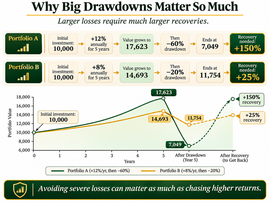
Consider two hypothetical portfolios.
Portfolio A earns 12% annually for five years before suffering a 60% decline.
Portfolio B earns 8% annually over the same five years before declining 20%.
Assuming the stated returns compound annually and there are no additional contributions, taxes, or fees:
| Portfolio A | Portfolio B | |
|---|---|---|
| Initial investment | €10,000 | €10,000 |
| Value after five years | €17,623 | €14,693 |
| Subsequent drawdown | −60% | −20% |
| Value after drawdown | €7,049 | €11,754 |
| Gain required to recover | +150% | +25% |
Despite Portfolio A’s superior returns during the preceding five years, its larger drawdown leaves the investor substantially worse off.
The example is deliberately simplified.
It does not imply that lower-volatility portfolios always produce better long-term results.
But it illustrates an important principle: avoiding severe losses can be as important to long-term wealth accumulation as generating attractive returns during favourable markets.
This becomes particularly relevant for investors who may need to withdraw capital, rebalance under constraints, or face financial obligations during a market downturn.
The ability to remain invested through difficult periods is itself a valuable characteristic of a portfolio.
Can an All-Seasons Portfolio Protect Against Every Crash?
No.
And any investment strategy claiming otherwise deserves scepticism.
An All-Seasons Portfolio can experience losses during financial crises, periods of rapidly rising interest rates, or other unexpected developments.
The last time that happened was in 2022, when stocks, government bonds and gold all fell together when central banks across the world rapidly raised rates, affecting even most portfolios/funds employing all-weather type strategies.
Diversification may reduce risk, but it cannot eliminate it.
Even assets that are economically distinct can temporarily become correlated during periods of extreme market stress.
The value of the approach lies elsewhere.
By combining assets with different sensitivities to growth, inflation, interest rates, and other economic forces, investors can reduce their dependence on a single market or economic scenario.
This can potentially produce a smoother investment experience and more balanced exposure to uncertainty.
However, the results depend on implementation.
Asset selection, portfolio weights, leverage, rebalancing, transaction costs, and changing market relationships all matter.
An All-Seasons strategy should therefore be understood as a framework for managing uncertainty, not a guarantee of protection.
The Greatest Risk May Be Believing We Understand Risk
Brazil’s October 2026 crash was extraordinary.
But the more important lesson is not that Brazilian equities are uniquely dangerous.
It is that financial markets repeatedly produce outcomes that simplistic statistical models struggle to explain.
The same phenomenon has appeared in developed equity markets, quantitative investment strategies, and global financial crises.
These events should encourage investors to question their assumptions.
Historical volatility is not a complete measure of risk.
Correlation is not constant.
Owning many securities does not necessarily mean owning genuinely different economic exposures.
And sophisticated models cannot replace sound economic judgement.
The purpose of diversification is not to predict every crisis.
It is to acknowledge that crises will occur, often in forms we did not anticipate.
An investor who accepts this uncertainty can construct a portfolio that is less dependent on being right about the future.
That is the philosophy behind All-Seasons investing.
We cannot make the unexpected disappear. But we can avoid building portfolios that assume it never happens.
Explore the AllSeasonsPort Strategy on etoro
At AllSeasonsPort on etoro, I apply these principles through a diversified, multi-asset investment approach inspired by All-Weather and risk parity investing, and have done so since 2021.
The strategy focuses on balancing exposure to different economic environments rather than relying exclusively on the performance of a single equity market.
My objective is to build a portfolio that can participate in long-term market growth while maintaining a disciplined approach to diversification and risk management.
If you’re interested in seeing how these principles translate into an actual investment portfolio, you can follow my investment activity and portfolio updates on etoro. You can even copy my portfolio to get an automatic exposure to an all-weather style portfolio.
Explore AllSeasonsPort on etoro
You can also follow my regular market commentary, where I discuss macroeconomic developments, cross-asset relationships, and portfolio construction.
Disclaimer: This article is provided for educational and informational purposes only and does not constitute investment advice or a personal recommendation. Investing involves risk, including the possible loss of capital. Diversification does not guarantee profits or protect against all losses. Past performance is not indicative of future results. Copy trading does not amount to investment advice, and the value of investments may rise or fall.
Sources and Further Reading
Brazil’s October 2026 market crash
- ETF.com — Brazil ETF Plunges Nearly 20% After Lula’s Surprise Win (26 October 2026).
- Reuters — Analysts Forecast Brazil Market Plunge After Lula Turnaround Win (26 October 2026).
Historical market crashes and statistical risk
- Federal Reserve History — Stock Market Crash of 1987.
- Stock, J. H. and Watson, M. W. — Introduction to Econometrics, discussion of the 1987 crash and the normal distribution.
- United Nations Conference on Trade and Development — Coping with Globalized Finance: Recent Challenges and Long-term Perspectives (2007), including discussion of the quantitative investment losses of August 2007.
Portfolio construction and diversification
- Bridgewater Associates — The All Weather Story.
- Bridgewater Associates — Engineering Targeted Returns and Risks (2011).
- PanAgora Asset Management — Risk Parity Portfolios: Efficient Portfolios Through True Diversification.
- Howard Marks — Uncertainty.
These materials provide additional context on portfolio diversification, risk balancing, uncertainty, and the limitations of conventional approaches to measuring investment risk.


